Stress vector

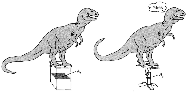
Consider two blocks of different cross-sections. Intuitively, the blocks whose cross-section is smaller is going to deform a lot more than the other. While in rigid body mechanics, the concept of force is sufficient to describe or predict the motion of the body, in deformable bodies it is not.

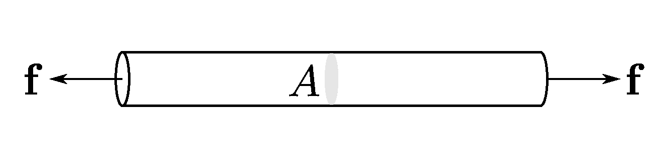
We will need to understand the concept of stress. The term stress (\(\sigma\)) is used to express the loading in terms of force applied to a certain cross-sectional area of an object.

From the perspective of loading, stress is the applied force or system of forces that tends to deform a body.

From the perspective of what is happening within a material, stress is the internal distribution of forces within a body that balance and react to the loads applied to it. The stress distribution may or may not be uniform, depending on the nature of the loading condition.

Traction

Simplifying assumptions are often used to represent force acting on area as traction vector - simply the force vector divided by that area.

\[\mathbf{t} = \frac{\mathbf{f}}{A}\]

\(\mathbf{t}\) has units of stress, but as it is a vector, all the usual rules for vectors apply to it.

The unit of stress is Pascal [Pa] or Newtons per square meter [\(\frac{N}{m^2}\)]. A stress of 1 Pa is very small, for example, the load due to 1m of water is about 10\(^4\) Pa. So, in geology we often use metric prefixes:

• 1 hPa = 10\(^2\) Pa (hektopascal)

• 1 kPa = 10\(^3\) Pa (kilopascal)

• 1 MPa = 10\(^6\) Pa (megapascal)

• 1 GPa = 10\(^9\) Pa (gigapascal)

Other units are bar:

• 1 bar = 10\(^5\) Pa

• 1 kbar = 10\(^8\) Pa = 100 MPa

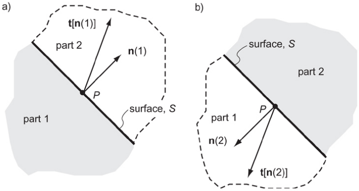
The traction is a vector quantity that acts at a point on an imaginary or real surface of arbitrary orientation.

Cauchy reciprocal theorem

The traction at a point on a surface is equal and opposite to the traction that at that same point for the same surface with opposite outward unit normal vector.

Stress components

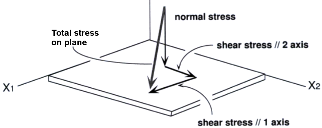
In general, a stress acting on a plane represented by traction \(\mathbf{t}\) may be expressed as a sum of shear and normal components.

\[\mathbf{t} = \boldsymbol{\sigma}_n + \boldsymbol{\tau}_{x_1} + \boldsymbol{\tau}_{x_1} = \boldsymbol{\sigma}_n + \boldsymbol{\tau}_n\]

Note

A normal component of the traction vector (\(\boldsymbol{\sigma}_n\)) acting perpendicular to the plane.

A shear component of the traction vector (\(\boldsymbol{\tau}_n\)) acting parallel to the plane.

The magnitude of the normal component \(\boldsymbol{\sigma}_n\) (i.e. normal stress) of any traction vector \(\mathbf{t}\) acting on an arbitrary plane with unit normal vector \(\mathbf{n}\) at a given point, could be calculated as it’s projection onto the unit normal vector, i.e. their scalar product:

\[\left| \boldsymbol{\sigma}_n \right| = \mathbf{t} \cdot \mathbf{n}\]

n = fol(150, 60)
t = 5 * vec('x')  # Traction vector oriented parallel to x-axis with magnitude 5
t.dot(n)  # normal stress magnitude (signed)

3.75

The vector representation of the normal component \(\boldsymbol{\sigma}_n\) could be expressed as unit normal vector scaled by a projection of the traction vector onto the unit normal vector:

\[\boldsymbol{\sigma}_n = (\mathbf{t} \cdot \mathbf{n})\mathbf{n}\]

sn = n*t.dot(n)  # scaled unit normal vector - normal stress
abs(sn)  # normal stress magnitude (always positive)

3.75

In APSG we can use vector projection:

sn = t.project(n)  # project traction vector t onto normal n - normal stress
abs(sn)  # normal stress magnitude (always positive)

3.75

The magnitude of shear component \(\boldsymbol{\tau}_n\) (i.e. shear stress), acting in the plane spanned by the two vectors \(\mathbf{t}\) and \(\mathbf{n}\), could be calculated as it’s rejection onto the unit normal vector, i.e. magnitude of their cross product:

\[\left| \boldsymbol{\tau} \right| = \left|\mathbf{t} \times \mathbf{n}\right|\]

abs(t.cross(n))  # shear stress magnitude (always positive)

3.3071891388307386

The shear component \(\boldsymbol{\tau}_n\), acting in the plane spanned by the two vectors \(\mathbf{t}\) and \(\mathbf{\sigma}_n\), can then be found as difference between traction vector \(\mathbf{t}\) and normal component \(\mathbf{\sigma}_n\):

\[\boldsymbol{\tau}_n = \mathbf{t} - \boldsymbol{\sigma}_n\]

or using the double cross product:

\[\boldsymbol{\tau}_n = \mathbf{n} \times (\mathbf{t} \times \mathbf{n})\]

tau = n.cross(t.cross(n))  # double cross product - shear stress
abs(tau)  # shear stress magnitude (always positive)

3.3071891388307386

In APSG we can use vector rejection:

tau = t.reject(n)  # reject traction vector t onto normal n - shear stress
abs(tau)  # shear stress magnitude (always positive)

3.307189138830738

Stress at point

It must be noted that the stresses in most 2-D or 3-D solids are actually more complex and need be defined more methodically.

The internal force acting on a small area of a plane represented by traction vector can be resolved into normal and shear stress components. These stresses are average stresses as the area is finite, but when the area is allowed to approach zero, the stresses become stresses at a point.

Since stresses are defined in relation to the plane that passes through the point under consideration, and the number of such planes is infinite, there appear an infinite set of stresses at a point.

Fortunately, it can be proven that the stresses on any plane can be computed from the stresses on three orthogonal planes passing through the point. This will bring us to the definition of the stress tensor…