Kinematics of continuum body

The motion of a continuum body is a continuous time sequence of displacements. Thus, the material body will occupy different configurations at different times so that a particle occupies a series of points in space which describe a pathline. There is continuity during deformation or motion of a continuum body in the sense that:

• The material points forming a closed curve at any instant will always form a closed curve at any subsequent time.

• The material points forming a closed surface at any instant will always form a closed surface at any subsequent time and the matter within the closed surface will always remain within

Kinematics: deformation and motion

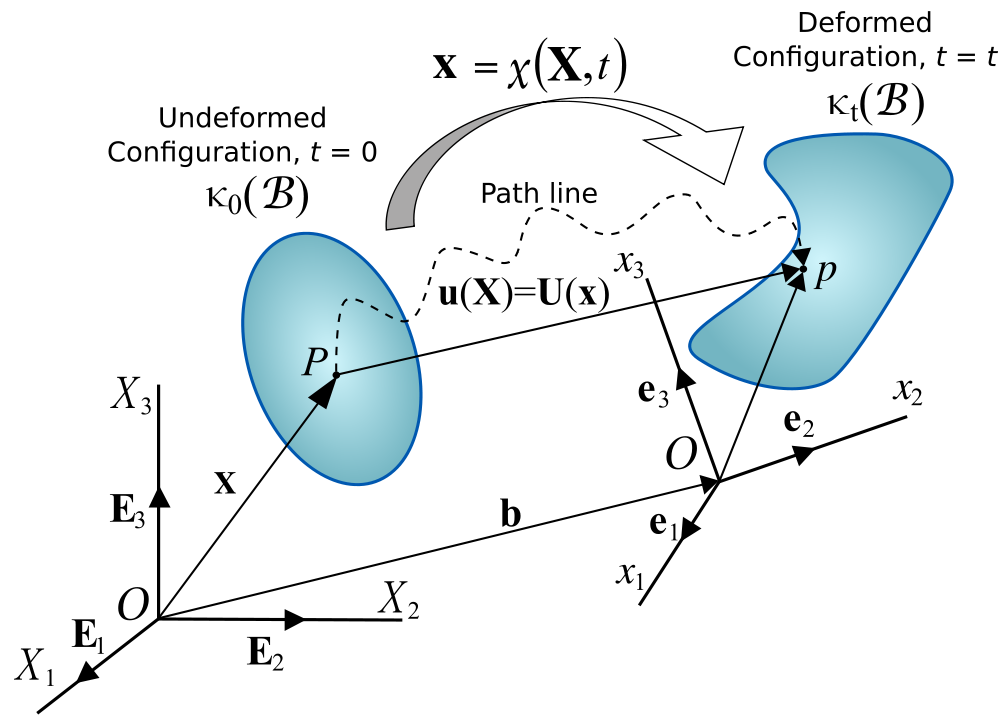
It is convenient to identify a reference configuration or initial condition which all subsequent deformed configurations are referenced from. Often, the configuration at \(t=0\) is considered the reference configuration.

The components \(x_i\) of the position vector \(\mathbf{x}\) of a particle, taken with respect to the reference configuration, are called the material or reference coordinates.

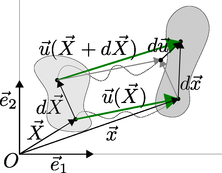
The displacement of first point is decribed as:

\[\mathbf{x} = \mathbf{X} + \mathbf{u}(\mathbf{X})\]

while displacement of second surrounding point is described as:

\[\mathbf{x} + d\mathbf{x} = \mathbf{X} + d\mathbf{X} + \mathbf{u}(\mathbf{X} + d\mathbf{X})\]

Substituting first equation into second we got:

\[\mathbf{X} + \mathbf{u}(\mathbf{X}) + d\mathbf{x} = \mathbf{X} + d\mathbf{X} + \mathbf{u}(\mathbf{X} + d\mathbf{X})\]

which simplifies to:

\[ d\mathbf{x} = d\mathbf{X} + \mathbf{u}(\mathbf{X} + d\mathbf{X}) - \mathbf{u}(\mathbf{X})\]

Taylor’s theorem

Taylor’s theorem states that any function that is infinitely differentiable may be represented by a Taylor series expansion:

\[f(X+dX)=f(X)+{\frac {f^{\prime }(X)}{1!}}dX+{\frac {f^{{\prime \prime }}(X)}{2!}}dX^{2}+...=\sum _{{k=0}}^{{\infty }}{\frac {f^{{(k)}}(X)}{k!}}dX^{{k}}\]

than

\[f(X+dX) - f(X) = {\frac {f^{\prime }(X)}{1!}}dX+{\frac {f^{{\prime \prime }}(X)}{2!}}dX^{2}+...=\sum _{{k=0}}^{{\infty }}{\frac {f^{{(k)}}(X)}{k!}}dX^{{k}}\]

neglecting higher terms as \(\left | d\mathbf{X} \right | \ll 1\) as \(dX^{{k}}\) is very small (we explore infinitesimal volume), it is:

\[ f(X+dX) - f(X) \approx {\frac {f^{\prime }(X)}{1!}}dX \]

Similarily (for details you have to dig into your math classes notes), for vector-valued functions we can write:

\[\mathbf{u}(\mathbf{X} + d\mathbf{X}) - \mathbf{u}(\mathbf{X}) \approx \boldsymbol{J}(\mathbf{u})d\mathbf{X}\]

where \(\boldsymbol{J}(\mathbf{u})\) is Jacobian matrix and in strain analysis, we usually called displacement gradient and we use symbol \(\boldsymbol{\nabla u}\). Using that for infinitesimal deformation equation:

\[d\mathbf{x} = d\mathbf{X} + \mathbf{u}(\mathbf{X} + d\mathbf{X}) - \mathbf{u}(\mathbf{X})\]

it could be written in terms of gradient as:

\[d\mathbf{x} = d\mathbf{X} + (\boldsymbol{\nabla u})d\mathbf{X}\]

where \(\boldsymbol{\nabla u}\) is gradient of displacement field or displacement gradient.

Displacement gradient

The displacement gradient is the matrix of all first-order partial derivatives of each component of the element displacement \(d\mathbf{u}\) with respect to each component of the reference element \(d\mathbf{X}\):

\[\begin{split}\boldsymbol{\nabla u} = u_{i,j} = \frac{\partial u_i}{\partial X_j} = \begin{bmatrix} \frac{\partial u_1}{\partial X_1} & \frac{\partial u_1}{\partial X_2} & \frac{\partial u_1}{\partial X_3} \\ \frac{\partial u_2}{\partial X_1} & \frac{\partial u_2}{\partial X_2} & \frac{\partial u_2}{\partial X_3} \\ \frac{\partial u_3}{\partial X_1} & \frac{\partial u_3}{\partial X_2} & \frac{\partial u_3}{\partial X_3} \end{bmatrix}\end{split}\]

and characterise the local change of the displacement field at a material point with position vector \(\mathbf{X}\). Knowing that:

\[d\mathbf{u} = d\mathbf{x} - d\mathbf{X}\]

it could be also written as:

\[d\mathbf{u} = (\boldsymbol{\nabla u})d\mathbf{X}\]

Deformation gradient

Recalling that \(d\mathbf{u} = d\mathbf{x} - d\mathbf{X}\)

\[(\boldsymbol{\nabla u}) = \frac{\partial u_i}{\partial X_j} = \frac{\partial (x_i - X_i)}{\partial X_j} = \frac{\partial x_i}{\partial X_j} - \frac{\partial X_i}{\partial X_j} = \boldsymbol{F} - \boldsymbol{I}\]

where \(\boldsymbol{F}\) is so called deformation gradient, i.e the derivative of each component of the deformed linear element \(d\mathbf{x}\) with respect to each component of the reference element \(d\mathbf{X}\):

\[\begin{split} \boldsymbol{F} = x_{i,j} = \frac{\partial x_i}{\partial X_j} = \begin{bmatrix} \frac{\partial x_1}{\partial X_1} & \frac{\partial x_1}{\partial X_2} & \frac{\partial x_1}{\partial X_3} \\ \frac{\partial x_2}{\partial X_1} & \frac{\partial x_2}{\partial X_2} & \frac{\partial x_2}{\partial X_3} \\ \frac{\partial x_3}{\partial X_1} & \frac{\partial x_3}{\partial X_2} & \frac{\partial x_3}{\partial X_3} \end{bmatrix}\end{split}\]

and characterizes the local deformation at a material point with position vector \(\mathbf{X}\), assuming continuity. Knowing that:

\[d\mathbf{x} - d\mathbf{X} = d\mathbf{u} = (\boldsymbol{\nabla u})d\mathbf{X} = (\boldsymbol{F} - \boldsymbol{I})d\mathbf{X} = \boldsymbol{F}d\mathbf{X} - d\mathbf{X}\]

it could be also written as:

\[d\mathbf{x} = \boldsymbol{F}d\mathbf{X}\]

Properties of deformation gradient

Deformation gradient \(\boldsymbol{F}\) contains all the required local information about the changes in length, volumes and angles due to the deformation as follows:

• When vector \(\mathbf{X}\) in the reference configuration is deformed into the vector \(\mathbf{x}\), these vectors are related as: \(\mathbf{x} = \boldsymbol{F}\mathbf{X}\)

• The Jacobian of the deformation gradient is equal to the ratio between the local volume of the deformed configuration to the local volume in the reference configuration i.e. volume change: \(J = \frac{dV}{dV_0} = \det({\boldsymbol{F})}\)

• Two infinitesimal areas with \(da\) and \(dA\) being their magnitudes and \(\mathbf{n}\) and \(\mathbf{N}\) are unit vectors perpendicular to them, then the relationship is given by: \((da)\mathbf{n} = \det(\boldsymbol{F})(dA)\boldsymbol{F}^{-T}\mathbf{N}\)

• An isochoric deformation is a deformation preserving local volume, i.e., \(\det({\boldsymbol{F}})=1\)

• A deformation is called homogeneous if \(\boldsymbol{F}\) is constant at every point. Otherwise, the deformation is called non-homogeneous

• The physical restriction of possible deformation: \(\det({\boldsymbol{F}}) > 0\)